if(!("maps" %in% row.names(installed.packages()))){install.packages("maps")}
if(!("mapproj" %in% row.names(installed.packages()))){install.packages("mapproj")}
if(!("mapdata" %in% row.names(installed.packages()))){install.packages("mapdata")}Class 10 notes
Packages
For personal projects, I like to use this to ensure that moving between computers and such, I have the packages I need. Unpacking it from the inside out is helpful for understanding how it works. Essentially, if the package name I think I will need is not in the list of installed packages, I install it.
Now load the packages, for some reason, mapdata didn’t like being listed with the others.
library(maps, mapproj)
library(mapdata)
library(ggplot2)
Selecting available data
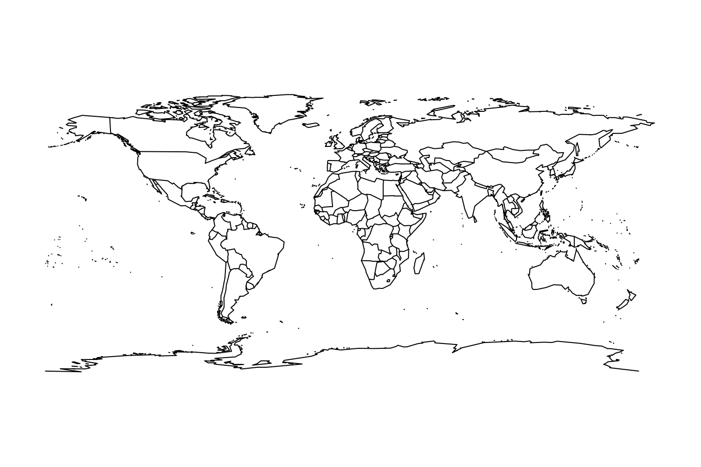
We can make a world map in Figure 1 using the command map(). Taking in no additional arguments, by defaults it will produce a dull world map.
Setting database = 'state' will give a United States map of the lower 48 states, as in Figure 2.
map(database = 'state')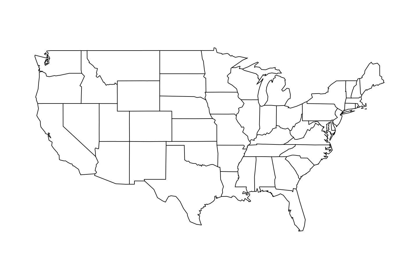
Making the same type of change, this time to a value of 'county', we get a county map as in Figure 3. For a little flourish, we first plot the county boundaries in gray, and overplot black state boundaries. This shows the tremendous variability, on average, of county area as you move East to West. There are 30 counties, mostly out West, with areas larger than the entire state of New Hampshire. More on that with a few special commands later.
map(database = 'county', col = "gray")
map('state', add = TRUE)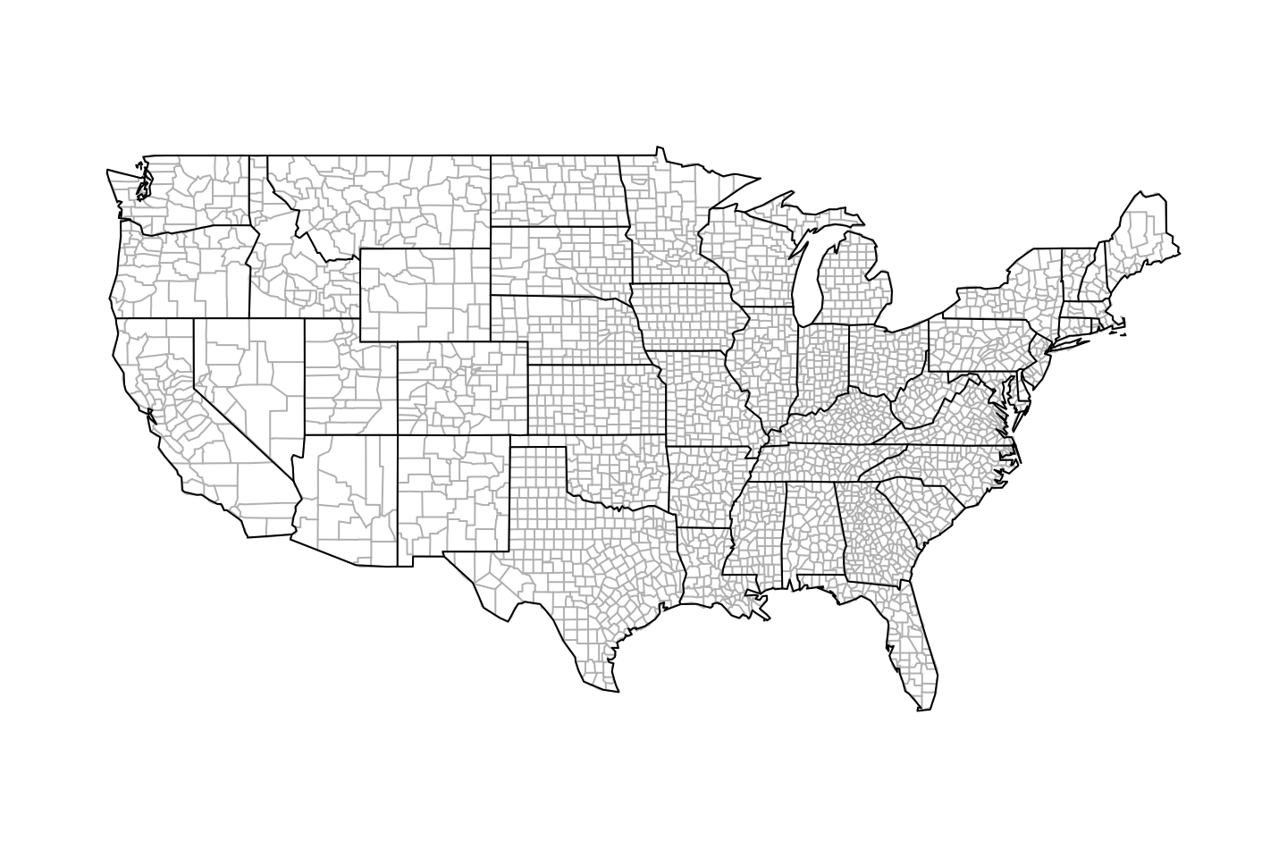
We can continue to “zoom in” by setting region = 'oklahoma'. There are a few things to note about the syntax for the map shown in Figure 4, first, or region is actually the state name, additionally it is spelled with all lowercase.
map(database = 'county', region = 'oklahoma')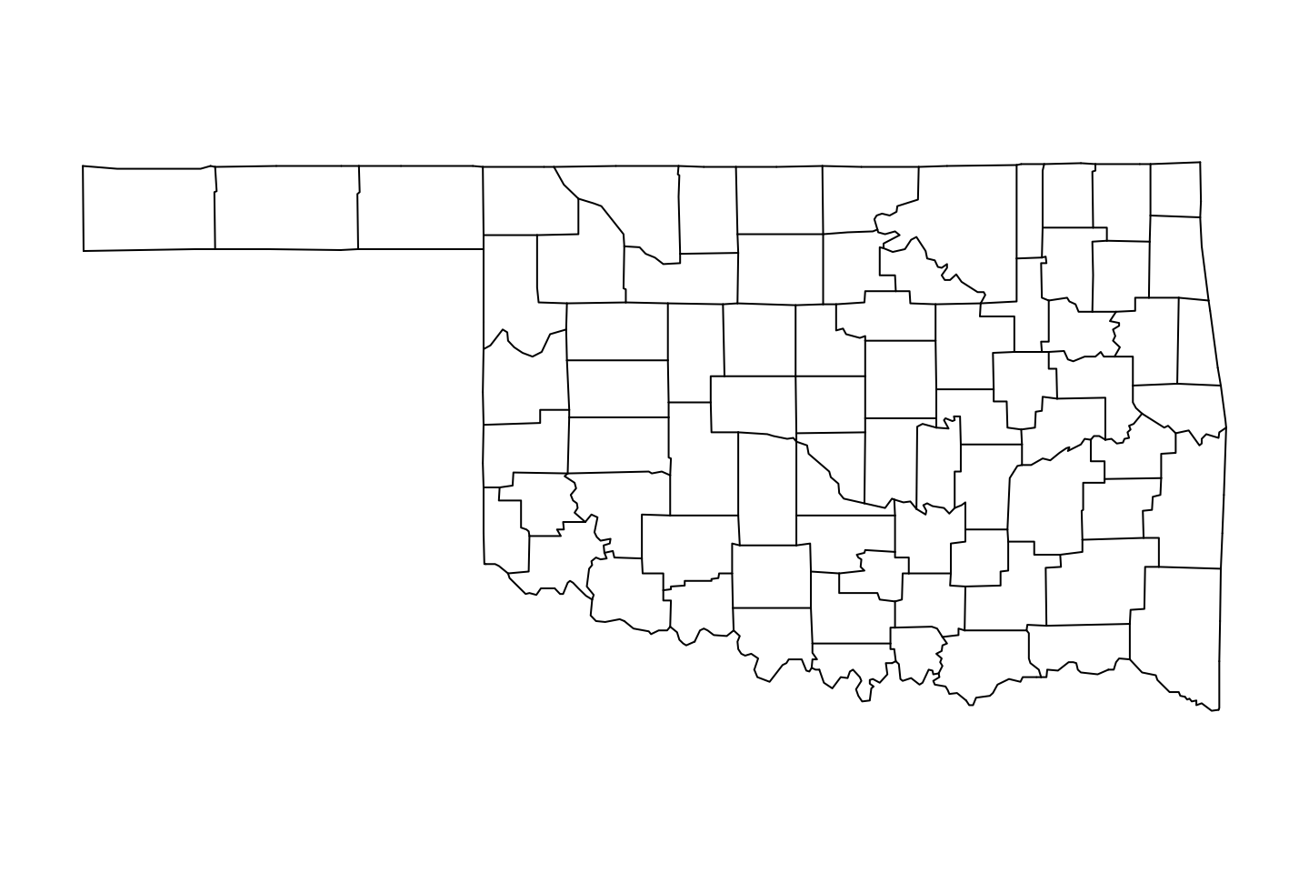
Color and creativity
After checking the help file for map(), we saw some background information about the region argument, in somewhat of an attempt to understand it, we tested a sample argumend involving the exclusion of Svalbard island from the map of Norway. After first making the map, we added a red fill on a skyblue background. To highlight the distinction between the two localities (ugh, “regions”) we overplot mainland Norway (“excluding” Svalbard Island) by highlighting with yellow. With a little work we should be able to add a suitable legend.
One sort of important idea here is that syntax to exclude Svalbard. That is based on Perl regular expressions. These can be used for incredibly powerful text editing/mining, but that would be the subject of nearly an entire day if not course.
par(bg = "skyblue")
map(region ="Norway", col = "red", fill = TRUE)
map(region ="Norway(?!:Svalbard)", col = "yellow", fill = TRUE, add = TRUE)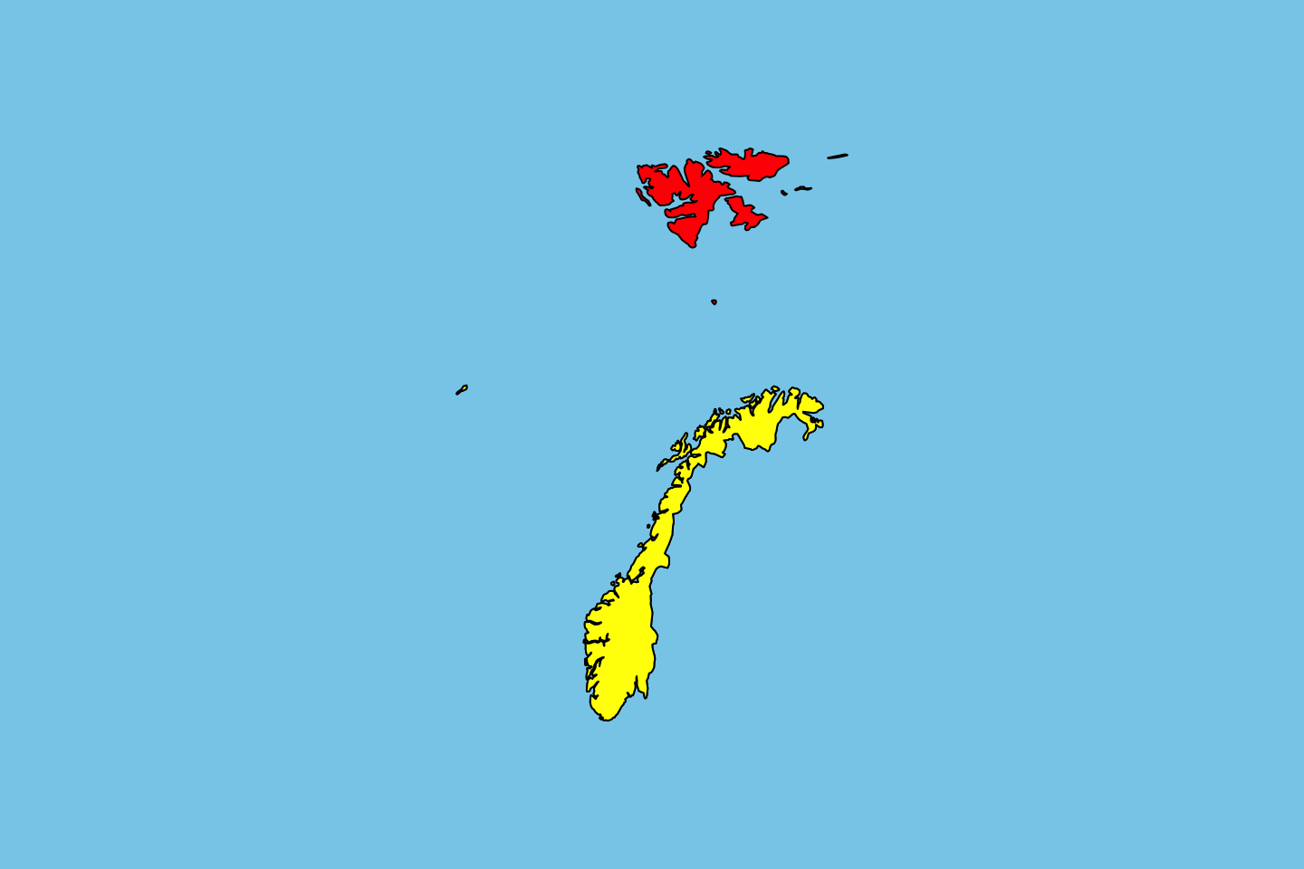
Interestingly enough, the above approach doesn’t seem to work for highlighting Chinese provinces. A failure seen in Figure 6.
par(bg = "skyblue")
map(region ="China", col = "red", fill = TRUE)
map(region ="China(?!:Qinghai)", col = "yellow", fill = TRUE, add = TRUE)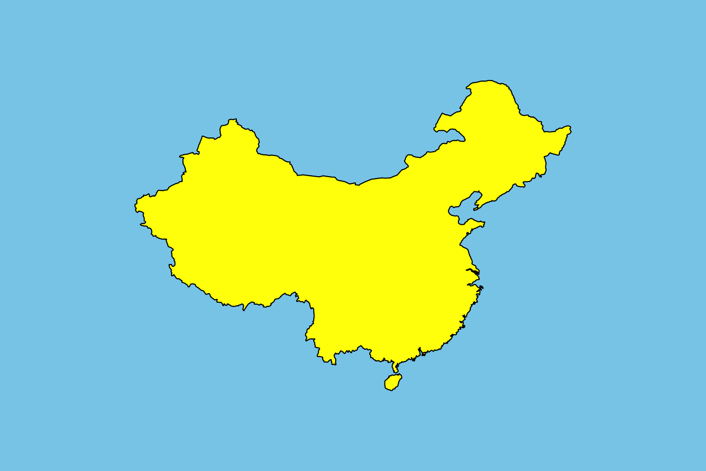
Maps as outlines
To perhaps better understand maps, we can look at the state outline data. To do so we will use the function map_data() from the ggplot2 library. It makes conveniently available the data for state outlines. A bit of investigation (creative use of tables, or simply reading the documentation) shows that the data shows latitude and longitude, group represents the spatial unit of a given state, or more generally its region.
usStates <- map_data("state")
plot(usStates[, c("long", "lat")], pch = 19, cex = 0.1, type = 'p')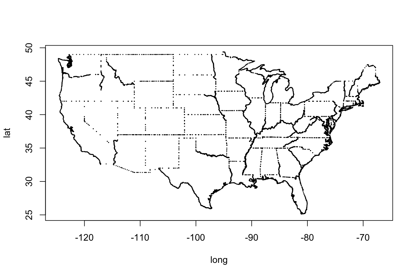
Had we set the argument of map_data() to "county", those names would fill subregion column. Now each county is a group. Not just disjoint lands like islands or detached peninsulas. The names region and subregion actually seem like great argument names after some thought.
To understand some of the additional variables a bit better, on-the-fly, we made a plot of the outline of Colorado, a simple (it sure seems) rectangle. By rotating the entries of order by 45 degrees, we can read the numbers a bit better and confirm that the maps is essentially “connect-the-dots” on a state-by-state basis.
plot(usStates[usStates$region == "colorado", c("long", "lat")], pch = 19, cex = 0.5, type = 'p')
text(usStates[usStates$region == "colorado", "long"], usStates[usStates$region == "colorado", "lat"], usStates[usStates$region == "colorado", "order"], srt = 45)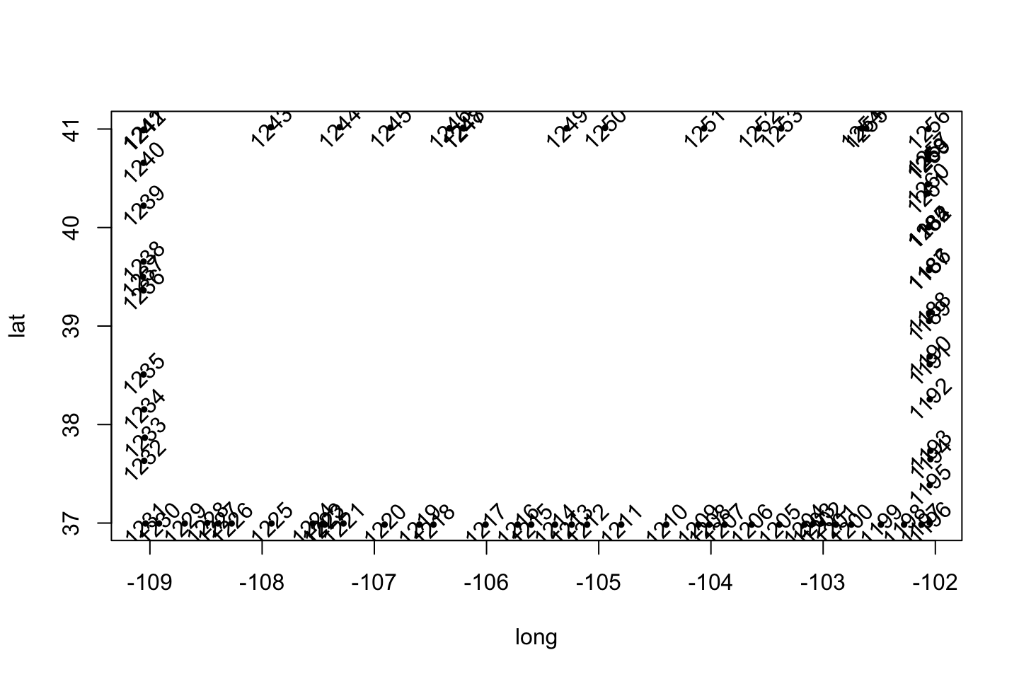
A more interesting example might be a state like Washington, or North Carolina. Again, make a state-by-state table of group numbers to see why. As Figure 9 confirms, the outline of Washington is created by five froups of points. In this more interesting case, it seems more helpful to color points by group rather than label points by order, as we had done in class.
cols <- usStates[usStates$region == "washington", "group"]; cols <- cols - min(cols) + 1
plot(usStates[usStates$region == "washington", c("long", "lat")], pch = 19, cex = 0.5, type = 'p', col = cols)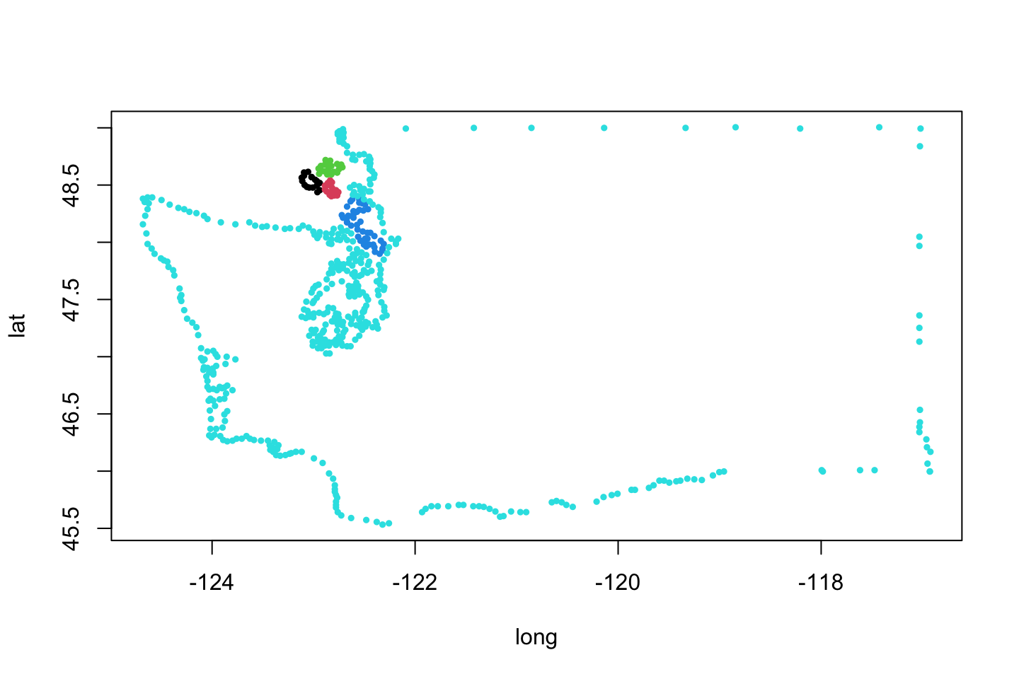
Given that data, we can use the code printed with Figure 10 to plot a map. Our approach is to plot the map as a collection of filled polygons. Interestingly, the seemingly redundant group = group argument, plays a large role. If we omit it, states with more than one land mass will be drawn having those land masses connected in odd ways.
ggplot(data = usStates,
       mapping = aes(x = long, y = lat,
       group = group, fill = region)) +
       geom_polygon(color = "black", linewidth = 0.1) +
       guides(fill = FALSE)
Warning: The `<scale>` argument of `guides()` cannot be `FALSE`. Use "none" instead as
of ggplot2 3.3.4.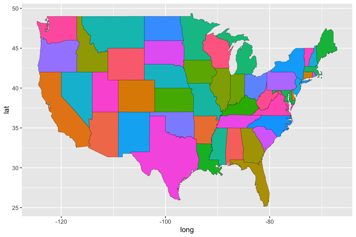
To be clear about the code, there is an argoment to ggplot() called mapping, this has nothing to do with the fact that we are map-making. This refers to the mapping of data to various properties of the eventual graph (e.g., soze, color, style, shape, depending, in general, on the geometry). The effect of this small change, not plotting by groups within states, is interesting (procedurally). But, as Figure 11 shows, it is also completely wrong. As the polygons intersect the filled regions reverse. This is the more colorful effect of what we saw with Figure 7 when we set type = 'l'.
ggplot(data = subset(usStates, region == "washington"),
       mapping = aes(x = long, y = lat,
       fill = "pink")) +
       geom_polygon(color = "black", linewidth = 0.1) +
       guides(fill = FALSE)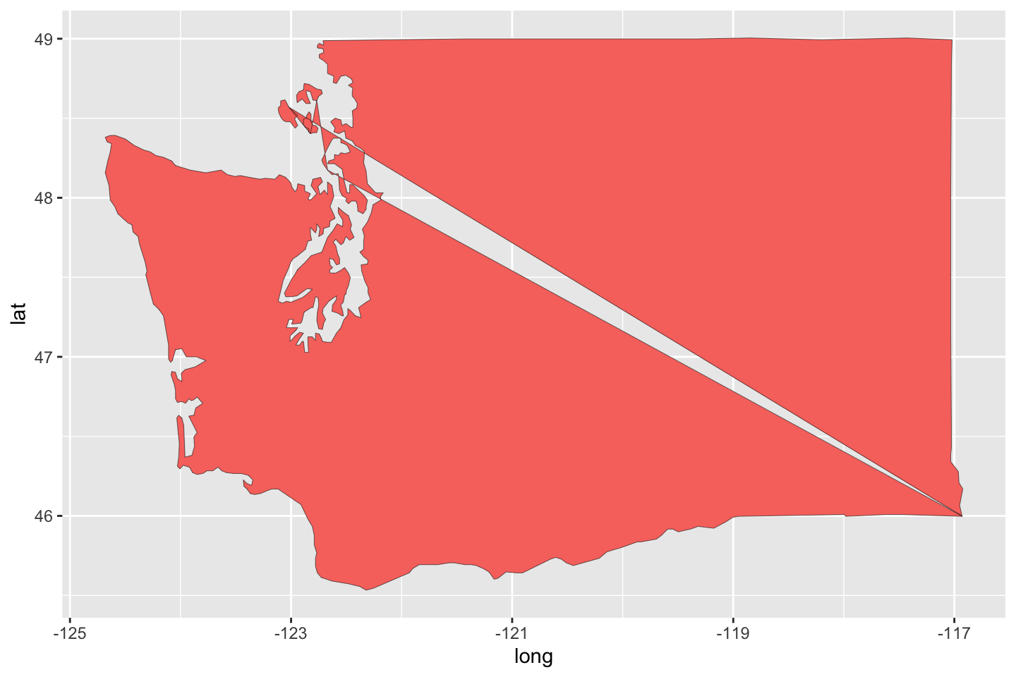
Having learned a bit more about syntax, we can do a bit to improve the appearance by turning to a more accepted map projection. The function coord_map() with arguments as shown allows us to change to one of many projections, some with their own necessary arguments, like lat0 and lat1. These change the scaling a bit, but it would require some systematic experimentation or careful reading to get a feel for their roles. They seem like acceptable choices based on existing books and work by experts in the field.
ggplot(data = usStates,
       mapping = aes(x = long, y = lat,
       group = group, fill = region)) +
       geom_polygon(color = "black", linewidth = 0.1) +
       coord_map(projection = "albers", lat0 = 39, lat1 = 45) +
       guides(fill = FALSE)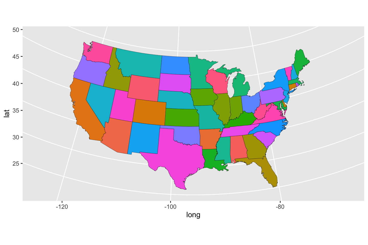
Sensible map coloring
Now we can start the real work. By importing a second set of data here describing the results of a survey on regional variation in drink terminology, we can color states using elements of the data. Read more about the survey1
dat <- read.delim("./data/drink-names.csv", header = TRUE, sep = '\t')
head(dat)
Region pop soda coke other Total Percent
1 Total 157659 164145 58490 21120 401414 100.00
2 Alabama 153 582 2849 665 4249 1.06
3 Alaska 324 636 60 92 1112 0.28
4 Alberta 2185 69 55 48 2357 0.59
5 American Samoa 8 11 1 40 60 0.01
6 Arizona 586 2799 437 174 3996 1.00The datasets share the identifier of state name, called "region" in the state map data and "Region" in the survey data. These datasets (or arbitrary columns of them) can be merged together by looking where the rows match in the name of the state. While it would have been just as easy to open the file and change case on either one of those, this is a nice opportunity to illustrate the flexibility of merge(). Since we are overwriting the original map data variable, just be careful not to execute this column more than onece in sequence or you will re-merge additional copies of the survey data to teh original data and accumulate appended .x, .y, or worse .x.y and so on. The easy fix is then just to start over by redefining the original merged object a few steps back. By merging in this direction we assign all survey values to each component of the state outline data. To match, we begin by converting the case of the actual entries, so that Alabama will match with alabama, and so on. Strangely the variable names as well as their entries differed in case.
dat$Region <- tolower(dat$Region)
usStates <- merge(usStates, dat, by.x = "region", by.y = "Region")
head(usStates)
region long lat group order subregion pop soda coke other Total
1 alabama -87.46201 30.38968 1 1 <NA> 153 582 2849 665 4249
2 alabama -87.48493 30.37249 1 2 <NA> 153 582 2849 665 4249
3 alabama -87.52503 30.37249 1 3 <NA> 153 582 2849 665 4249
4 alabama -87.53076 30.33239 1 4 <NA> 153 582 2849 665 4249
5 alabama -87.57087 30.32665 1 5 <NA> 153 582 2849 665 4249
6 alabama -87.58806 30.32665 1 6 <NA> 153 582 2849 665 4249
Percent
1 1.06
2 1.06
3 1.06
4 1.06
5 1.06
6 1.06The fact that there is one line of survey values per state means that those values repeat for each data point corresponding to a point on the boundary of each state – that is over 1000 points for Texas, with a large size and complicated perimeter. The duplication does not cause harm here, and it is an unavoidable step in specifying aes().
Though this does not make the best or most interesting use of the data, we can color by the statewide percent of the total population who responded as survey participants – this give no information about their actual answer in terms of preference. Ultimately we might care more about their answers, but this builds a good example. The percent participating colors each state, with an automatically generated color scheme. By comparing the map in Figure 13 to data – always a good idea, it’s too easy to make mistakes, misinterpret a value in data, or miss out on an opportunity to learn something – we can verify, in the absence of a legend, that darker colors are lower percents and brighter colors are higher.
ggplot(data = usStates,
  mapping = aes(x = long, y = lat,
  group = group, fill = Percent)) +
  geom_polygon(color = "gray90", linewidth = 0.1, show.legend = TRUE) +
  coord_map(projection = "albers", lat0 = 39, lat1 = 45) +
  guides(fill = FALSE)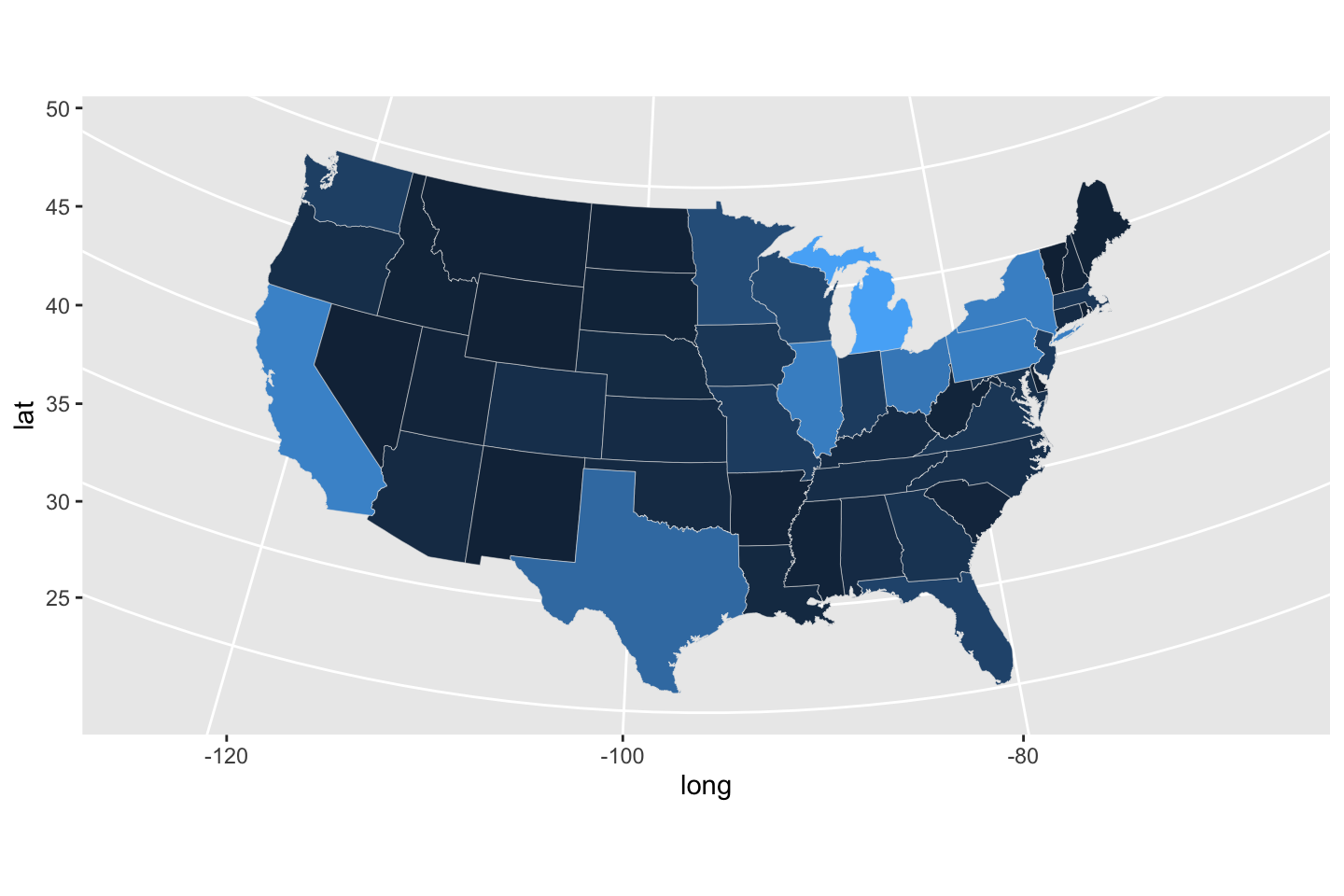
There were a lot of only slightly different colors in Figure 13, which did not necessarily help. We our readers could get distracted by too subtle of details, perhaps. For simplicity we will omit the first line of data, which actually correspnds to the marginal summary. It is easy to recreated this with apply(dat[, -1], 2, sum). We would not be able to calculate the mean of the first column, words, so we omit it with the syntax [, -1]. Visual analysis of the basic histogram, suggests, if only for the purposes of interpretation, we could look at binning the percent values at each even percent up to \(5\%\) and then possibly having a “catch-all” category like “\(>5\%\)”.
dat <- dat[-1, ]
hist(dat$Percent)
##head(dat)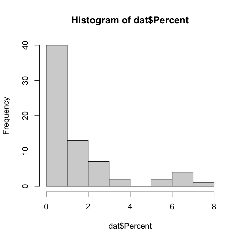
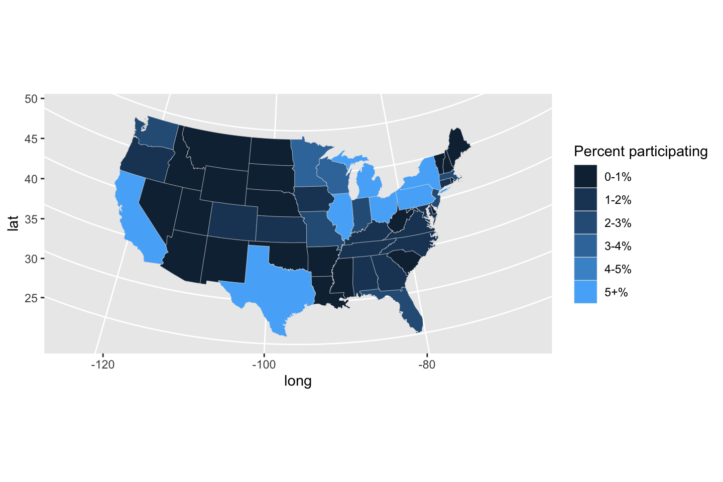
It’s worth experimenting with the layers of commands in the first line, but essentially cut() is a very slick way to decide which bin each value belongs to. Essentially this converts a number into a category. The resultung variable, bin, can be used to color. Explore with the bin spacings, perhaps every \(2\%\) from \(0\%\) to \(10\%\), since in this data nothing exceeds \(10%\) and that might seem like an intuituve cutoff. There is not a rule for making this decision. Look at data on the side, in a number of ways, avoid choices you would have a hard time explaining, and be honest about what you see.
usStates$bin2 <- cut(usStates$Percent, c(0, 1, 2, 3, 4, 5, 100))
usStates$bin <- as.numeric(usStates$bin2)

ggplot(data = usStates,
  mapping = aes(x = long, y = lat,
  group = group, fill = bin)) +
  geom_polygon(color = "gray90", linewidth = 0.1, show.legend = TRUE) +
  coord_map(projection = "albers", lat0 = 39, lat1 = 45) +
  scale_fill_continuous(
#    labels = levels(usStates$bin2),
    labels = c("0-1%","1-2%", "2-3%", "3-4%", "4-5%", "5+%"),
    guide = guide_legend(title = "Percent participating")
  )
The controversy
Ideally we would soon start looking at coloring using actual interesting values in the data. But, to avoid the xkcd “all maps are just population maps” pitfall (change fill = bin to fill = Total above to get a sense of what the population map would look like.), we wouldn’t want to use any of the raw vote numbers. We would want to convert them to something like “per 100,000” to standardize. Even then there are issues with other kinds of data where, for good reasons, like privacy, certain data, like suicide incidences, are not even included in certain published reports because in small populations that information could become personally-identifiable. One reasonable strategy would be to look at shares of the vote. With transparency you could possibly layer maps with contrasting, but pleasantly and perceptibly overlapping colors or filled contours. Or, variations on faceting or small-multiples with beverage-as-panl.
Go experiment. As you can see, making the maps alone was a task, now carefully superimposing or incorporating spatial data becomes the next step.