#dat <- read.delim("./data/cards.csv", header = TRUE, sep = ',')
tab <- table(warpbreaks$wool)
tab2 <- table(warpbreaks[, c("wool", "tension")])
tab2 <- as.data.frame(tab2)Class 5 notes
Data Visualization and Exploration
Unleashed
Read in one or more of the data sets and start using commands from class to explore.
Cautious first steps
The dataset warpbreaks is hopefully familiar by now. Here we don’t even have to read anything in, but might was well leave that as a reminder. It doesn’t take up much space.1
There is a difference between the objects created in the last two lines above. They contain exactly the same information, and the first is probably easier to understand. But the structure of the second, where all combinations are repeated as rows is a much better habit to build. You will thank yourself later.2
Sometimes it is useful to return some numerical summary for one variable across some combination of categories of related variables3. Below we will calculate the mean of a numerical measurement among members of collections of potentially related groups. You could list as many things as you wanted, by name4. The order just forces the order of columns, so you should pay close attention if columns have similar looking entries and one could be confused for another.
Below we’ll call the first one agg to pay homage to the aggregate() function. Then, agg2 could represent the 2D table, or more simply the second in a quick series of calculations where you want to take small steps. Trying to write the second of these as a data frame results in no change.
agg <- aggregate(warpbreaks$breaks, by = list(warpbreaks$wool), mean)
agg2 <- aggregate(warpbreaks$breaks, by = list(warpbreaks$wool, warpbreaks$tension), mean)
## no effect of the line below
## already a data frame
agg2.dat <- as.data.frame(agg2)
In reality the approach below is what I should have been doing all these years and I am rapidly trying to incorporate it into my work. That said, however you get started, you’ll be okay.
agg2b <- aggregate(breaks ~ wool + tension, warpbreaks, mean)To make this idea a little more useful, we can start to build little summary tables that are nicely formatted.
You can do this mostly by copy-and-paste. There’s really no harm in that. There are fancier tools and ways to come, but it’s really only a matter of what a couple of characters are and where you put them in the code. This is speedy enough and is quite transparent. We calculate all relevant cominations of statistics of interest, there could be more and we’d just repeat versions of the last two lines in sequence5
agg2b.mn <- aggregate(breaks ~ wool + tension,  warpbreaks, mean)
agg2b.sd <- aggregate(breaks ~ wool + tension,  warpbreaks, sd)
agg2b.mn <- merge(agg2b.mn, agg2b.sd, by = c("wool", "tension"))
You can simply repeat the last two of those lines for as many applied functions as you want. You could get quite creative6. If you even happened to have a larger object with the same classifiers, or even some combination7, and you can merge and maintain about anything. It’s really quite remarkable. When you’are all done with that, you just print the table to a file. There usually seem to be nothing harmful about setting row.names = TRUE, sometimes ugly rownames accumulate through an inefficient cycle of merge() and after aggregate() or after loadging the results of another dataset. Sometimes it’s nice to just say no.
write.table(agg2b.mn, "warpbreaks-summary.csv", sep = ",", col.names = TRUE, row.names = FALSE)Suppose out of habit I’d defined agg2 as above, I could get to the same point with the following code. Does this really matter? No. But its often nice to have a bunch of flexible ways to do the same thing. It makes you versatile. I grew up watching the original MacGyver8. Remember that agg2 was the version with the obscure variable names, to be clear, Group.1, Group.2, and x. The reminder here is that merge() is flexible.
It’s always nice to be able to rename things. In the event that to-be-merged variable names match, they’ll be dotted .x and .y accordingly, so it’s nice so to have a way to rename things regardless of how you approach certain steps. You can also rename any subset of variables [a:b] or even with reordering9 some subset (e.g., c(1, 9, 4) chosen by name or number). Please be careful, it might not give an error, but it might not make much sense either.
agg2.mn <- merge(agg2, agg2b.sd, by.x = c("Group.1", "Group.2"), by.y = c("wool", "tension"))
names(agg2.mn) <- c("wool", "tension", "mean", "sd")
I thought I could avoid iris but I couldn’t. In some circumstance for a quick calculation it was relatively helpful to compute and nicely organize and summary statistic of a few variables at a time across one category. Bebow the category is referenced as a name, but it could just as easily be done with the dollar sign (iris$Species) or the number (ugh, iris[5, ], I like the wordy variables first). This feels off to me, just by looking at it. I like keeping columns with different types of entries organized in groups - categorical or text-based first and numerical values after.
head(iris) Sepal.Length Sepal.Width Petal.Length Petal.Width Species
1 5.1 3.5 1.4 0.2 setosa
2 4.9 3.0 1.4 0.2 setosa
3 4.7 3.2 1.3 0.2 setosa
4 4.6 3.1 1.5 0.2 setosa
5 5.0 3.6 1.4 0.2 setosa
6 5.4 3.9 1.7 0.4 setosaaggregate(iris[ , 1:4], by = list(iris[, "Species"]), var) Group.1 Sepal.Length Sepal.Width Petal.Length Petal.Width
1 setosa 0.1242490 0.14368980 0.03015918 0.01110612
2 versicolor 0.2664327 0.09846939 0.22081633 0.03910612
3 virginica 0.4043429 0.10400408 0.30458776 0.07543265GROUP PROJECT TIME
To start wtih graphing, here is a reminder of using a par() argument for changing margins. This can be useful if you have long axis tick mark labels. As always, c(b, l, t, r).
par(mar = c(8.1, 4.1, 0.8, 0.8))
# plot(...)
Here goes. Experiment with and interpret the results of each of the following. You may have to execute them one at a time and either run as (tab <- table(warpbreaks$wool)), the parenthesis are a clever way to force printing after assignment, without having to call the result by name in the next line. But, this always confuses me in Quarto because it only prints the last text-based object of a code block (unless it has graphs).
tab <- table(warpbreaks$wool)
tab
 A  B
27 27
tab2 <- table(warpbreaks[, c("tension", "wool")])
tab2 <- table(warpbreaks[, c("breaks", "wool")])
tab2 <- table(warpbreaks[, c("tension", "wool")])
tab2 <- table(warpbreaks[, c("wool", "tension")])Those tables are each nice, but we can often make them more useful by turning the combinations into rows in a list instead of cells in a more complicated interaction. To me this is a Pro-Tip. In particular you can use this to generate as a piece of data to be merged with something else. Hint: it is very nice for checking combinations in dates from field notes to see if you didn’t lose or skip a page when digitizing.
tab2 <- as.data.frame(tab2)Since someone asked, if merging objects throughout a file, make sure they match. If you’ve modified naming conventions you can use by.x and by.y to specify whatever variable names you need for matching. If one has things the other doesn’t, you can use all.x = TRUE (same for all.y) or all (both) to control how many NA entries might clutter your screen. Experiment with this merging two different, but related, datasets that contain one or more common identifiers. The dim() command is useful to learn about the size of the objects you are creating through merging.
agg2 <- merge(agg2, agg2b.sd, by.x = c("Group.1", "Group.2"), by.y = c("wool", "tension"))We have a bunch of similar calculations laying around and have to be careful about the names. Weve used the . (‘dot’) and you could use camelCapping, but you can’t use - (‘dash’) because it is interpreted as subtraction, and probably shouldn’t use the _ (‘underscore’) because it is ugly. Once again we can rename some or all of the names of a data frame at any time.
names(agg2.mn) <- c("wool", "tension", "mean", "sd")Suppose that was to polish off a dataset for printing. We can use either line below to print. If we happen to have row names that we want, or do not, here might be our chance to make changes. In practice, I can only think of a time or two that this really mattered and it was usually only a matter of the difference of a couple of sed ... commands in the Terminal or Command Prompt.
write.table(agg2.mn, "warpbreaks-summary.csv", sep = ",", col.names = TRUE, row.names = FALSE)
write.table(agg2.mn, "warpbreaks-summary.csv", sep = ",", col.names = TRUE, row.names = TRUE)Iris10
I’d hoped to avoid using this data set, iris, but some times, some things are just to perfect. There are reasons everybody uses this data set, for one its nice to stop and thing about flowers every so often. Below we verify the structure of iris then conmite a variety of summary tables. These could all be saved or merged. If you were really fancy you could store a bunch of functions in a vector, put that in a loop, and proably automate that.
head(iris) Sepal.Length Sepal.Width Petal.Length Petal.Width Species
1 5.1 3.5 1.4 0.2 setosa
2 4.9 3.0 1.4 0.2 setosa
3 4.7 3.2 1.3 0.2 setosa
4 4.6 3.1 1.5 0.2 setosa
5 5.0 3.6 1.4 0.2 setosa
6 5.4 3.9 1.7 0.4 setosaaggregate(iris[ , 1:4], by = list(iris[, "Species"]), median) Group.1 Sepal.Length Sepal.Width Petal.Length Petal.Width
1 setosa 5.0 3.4 1.50 0.2
2 versicolor 5.9 2.8 4.35 1.3
3 virginica 6.5 3.0 5.55 2.0aggregate(iris[ , 1:4], by = list(iris[, "Species"]), sd) Group.1 Sepal.Length Sepal.Width Petal.Length Petal.Width
1 setosa 0.3524897 0.3790644 0.1736640 0.1053856
2 versicolor 0.5161711 0.3137983 0.4699110 0.1977527
3 virginica 0.6358796 0.3224966 0.5518947 0.2746501aggregate(iris[ , 1:4], by = list(iris[, "Species"]), length) Group.1 Sepal.Length Sepal.Width Petal.Length Petal.Width
1 setosa 50 50 50 50
2 versicolor 50 50 50 50
3 virginica 50 50 50 50aggregate(iris[ , 1:4], by = list(iris[, "Species"]), var) Group.1 Sepal.Length Sepal.Width Petal.Length Petal.Width
1 setosa 0.1242490 0.14368980 0.03015918 0.01110612
2 versicolor 0.2664327 0.09846939 0.22081633 0.03910612
3 virginica 0.4043429 0.10400408 0.30458776 0.07543265Convenience
In a question of convenience, it was asked how to more easily see, and store, the result of a calculation. I guess I should have said write name <- ...; name. But again outside of Quarto, using ( ... <- ...) works well. Since earlier we turned one of these tables into a data frame, I tried that here, and it didn’t matter because the original output was about as simplified as it could be.
agg <- aggregate(warpbreaks$breaks, by = list(warpbreaks$wool), mean)
(agg <- aggregate(warpbreaks$breaks, by = list(warpbreaks$wool), mean))
Group.1 x
1 A 31.03704
2 B 25.25926## no effect of the line below
## already a data frame
(agg2.dat <- as.data.frame(agg2)) Group.1 Group.2 x breaks
1 A H 24.55556 10.272671
2 A L 44.55556 18.097729
3 A M 24.00000 8.660254
4 B H 18.77778 4.893306
5 B L 28.22222 9.858724
6 B M 28.77778 9.431036The Mouse-Elephant curve
The primary challenge here is that the two numeric variables span a massive range. It would be great here to graph with a log scale. Time could be spent using text() with text positions calculated from rows in the data to annotate key points (i.e., animal names) of interest. Just for a reminder, the first line won’t work because the separation character needs to be specified. There are a variety of read.*() functions, so find your favorite.
While on the topic, there was a question about pasting strings, possibly for annotation. The goal was neat, but too specific for the moment. Just to toss out a suggestion for now, I would read ?plotmath, if that documentation exists, and experiment with every possible permutation of paste(), expression(), bquote(), and possibly parse(), or look for a suggested response to a related question on https://stackexchange.com and pick the one with the most of those words.
#mouse <- read.delim("./data/mouse.csv")
mouse <- read.delim("./data/mouse.csv", sep = ',')
paste(mouse$Animal, mouse$Mass)
[1] "Mouse 0.02" "Rat 0.2" "Guinea pig 0.8" "Cat 3"
[5] "Rabbit 3.5" "Dog 15.5" "Chimpanzee 38" "Sheep 50"
[9] "Human 65" "Pig 250" "Cow 400" "Polarbear 600"
[13] "Elephant 3670" Diabetes data
The diabetes data from https://github.com/datasets/diagnosed-diabetes-prevalence can be approached below. The file is in the corresponding class folder.
diabetes <- read.delim("./data/diabetes.csv", sep = ',')After using names(), head(), tail(), summary(), or even on a whim plot(), it’s time to make tables. After that initial exploration, we know that columns are "State" and "Year". We can make a table of the combinations of these that occur within the dataset. The results are rather interesting. Perhaps we should have known, but sometimes you forget, and sometimes there are some hidden assumptions within the structure of a dataset that you can easily overlook.
table(diabetes[, c("State", "Year")]) Year
State 2004 2005 2006 2007 2008 2009 2010 2011 2012 2013
\\Alaska 1 1 1 1 1 1 1 1 1 1
Alabama 65 65 65 65 65 65 65 65 65 65
Alaska 22 22 22 22 22 22 22 22 22 22
Arizona 15 15 15 15 15 15 15 15 15 15
Arkansas 72 72 72 72 72 72 72 72 72 72
California 58 58 58 58 58 58 58 58 58 58
Colorado 64 64 64 64 64 64 64 64 64 64
Connecticut 8 8 8 8 8 8 8 8 8 8
Delaware 3 3 3 3 3 3 3 3 3 3
District of Columbia 1 1 1 1 1 1 1 1 1 1
Florida 67 67 67 67 67 67 67 67 67 67
Georgia 137 137 137 137 137 137 137 137 137 137
Hawaii 5 5 5 5 5 5 5 5 5 5
Idaho 44 44 44 44 44 44 44 44 44 44
Illinois 102 102 102 102 102 102 102 102 102 102
Indiana 92 92 92 92 92 92 92 92 92 92
Iowa 99 99 99 99 99 99 99 99 99 99
Kansas 105 105 105 105 105 105 105 105 105 105
Kentucky 120 120 120 120 120 120 120 120 120 120
Louisiana 64 64 64 64 64 64 64 64 64 64
Maine 16 16 16 16 16 16 16 16 16 16
Maryland 24 24 24 24 24 24 24 24 24 24
Massachusetts 14 14 14 14 14 14 14 14 14 14
Michigan 83 83 83 83 83 83 83 83 83 83
Minnesota 87 87 87 87 87 87 87 87 87 87
Mississippi 82 82 82 82 82 82 82 82 82 82
Missouri 115 115 115 115 115 115 115 115 115 115
Montana 56 56 56 56 56 56 56 56 56 56
Nebraska 93 93 93 93 93 93 93 93 93 93
Nevada 17 17 17 17 17 17 17 17 17 17
New Hampshire 10 10 10 10 10 10 10 10 10 10
New Jersey 21 21 21 21 21 21 21 21 21 21
New Mexico 33 33 33 33 33 33 33 33 33 33
New York 62 62 62 62 62 62 62 62 62 62
North Carolina 100 100 100 100 100 100 100 100 100 100
North Dakota 53 53 53 53 53 53 53 53 53 53
Ohio 88 88 88 88 88 88 88 88 88 88
Oklahoma 77 77 77 77 77 77 77 77 77 77
Oregon 36 36 36 36 36 36 36 36 36 36
Pennsylvania 67 67 67 67 67 67 67 67 67 67
Puerto Rico 56 56 56 56 56 56 56 56 56 56
Rhode Island 5 5 5 5 5 5 5 5 5 5
South Carolina 46 46 46 46 46 46 46 46 46 46
South Dakota 66 66 66 66 66 66 66 66 66 66
Tennessee 93 93 93 93 93 93 93 93 93 93
Texas 220 220 220 220 220 220 220 220 220 220
Utah 27 27 27 27 27 27 27 27 27 27
Vermont 14 14 14 14 14 14 14 14 14 14
Virginia 132 132 132 132 132 132 132 132 132 132
Washington 37 37 37 37 37 37 37 37 37 37
West Virginia 51 51 51 51 51 51 51 51 51 51
Wisconsin 65 65 65 65 65 65 65 65 65 65
Wyoming 23 23 23 23 23 23 23 23 23 23diabetes2 <- as.data.frame(table(diabetes[, c("State", "Year")]))The outputs from the above lines (only the first one has been printed) are both equally useful in different ways. I don’t hate either. The one thing that they seemed to show is that at some point, one Alaskan City Council member (or the math professor that downloaded the file made a typo).
In all of this, it became clear that there was that typo. We can find it.
diabetes[diabetes$State == "\\Alaska", ] State FIPS_Code County Year Number Percent
70 \\Alaska 2100 Haines Borough 2004 97.0 5.7
3183 \\Alaska 2100 Haines Borough 2005 111.0 6.3
6296 \\Alaska 2100 Haines Borough 2006 114.0 6.5
9409 \\Alaska 2100 Haines Borough 2007 119.1 6.6
12522 \\Alaska 2100 Haines Borough 2008 118.3 6.6
15635 \\Alaska 2100 Haines Borough 2009 148.0 7.9
18748 \\Alaska 2100 Haines Borough 2010 163.0 8.3
21861 \\Alaska 2100 Haines Borough 2011 165.0 8.2
24974 \\Alaska 2100 Haines Borough 2012 140.0 7.0
28087 \\Alaska 2100 Haines Borough 2013 159.0 7.9
Lower_Confidence_Limit Upper_Confidence_Limit Age_Adjusted_Percent
70 3.8 8.0 5.0
3183 4.3 8.9 5.5
6296 4.3 9.3 5.9
9409 4.2 9.4 6.1
12522 4.3 9.6 6.1
15635 5.7 10.7 6.9
18748 6.1 11.0 6.8
21861 5.9 10.8 6.7
24974 5.0 9.3 5.7
28087 5.8 10.2 6.3
Age_Adjusted_Lower_Confidence_Limit Age_Adjusted_Upper_Confidence_Limit
70 3.4 7.1
3183 3.8 7.8
6296 3.9 8.3
9409 3.9 8.7
12522 4.0 8.9
15635 5.0 9.2
18748 5.0 9.0
21861 4.8 8.9
24974 4.1 7.6
28087 4.6 8.3Remember that the indexing of a data frame is [rows, columns], the rows and columns can be concatenated numbers, variable names, or sequences of numbers. Mostly I find myself doing logic to extract subsets of rows, and _carefully_ making slight adjustments to the order of columns at times. Below we inspect some incorectly-written entries of "\\Alaska", quite honestly I wondered if I accidentally added that while downloading the file.
diabetes[diabetes$State == "\\Alaska", "State"] [1] "\\Alaska" "\\Alaska" "\\Alaska" "\\Alaska" "\\Alaska" "\\Alaska"
[7] "\\Alaska" "\\Alaska" "\\Alaska" "\\Alaska"We can simultaneously overwrite those entries with the corrected encoding. I’m sure there are a lot of fancier tools, but I’ve learned a lot of hard lessons, faster this way and avoided negative consequequences of sloppy work. After overwriting those entries, we can test and see that nothing matches the original entry.
diabetes[diabetes$State == "\\Alaska", "State"] <- "Alaska"
diabetes[diabetes$State == "\\Alaska", ]
[1] State FIPS_Code
[3] County Year
[5] Number Percent
[7] Lower_Confidence_Limit Upper_Confidence_Limit
[9] Age_Adjusted_Percent Age_Adjusted_Lower_Confidence_Limit
[11] Age_Adjusted_Upper_Confidence_Limit
<0 rows> (or 0-length row.names)With that fixed, we’ll show the head of the data where State is California and Year is 2004. There was no specific reason for these choices, any other combination of place and time would have been sufficient. We will first look at all columns, then just the "Number" column.
head(diabetes[diabetes$State == "California" & diabetes$Year == 2004, ]) State FIPS_Code County Year Number Percent
176 California 6001 Alameda County 2004 73600 7.0
177 California 6003 Alpine County 2004 64 6.7
178 California 6005 Amador County 2004 2038 6.8
179 California 6007 Butte County 2004 9751 6.2
180 California 6009 Calaveras County 2004 2408 6.8
181 California 6011 Colusa County 2004 900 6.5
Lower_Confidence_Limit Upper_Confidence_Limit Age_Adjusted_Percent
176 5.5 8.6 7.2
177 4.4 9.7 6.5
178 5.1 9.0 5.9
179 4.8 8.0 5.8
180 5.1 9.0 5.7
181 4.8 8.8 6.4
Age_Adjusted_Lower_Confidence_Limit Age_Adjusted_Upper_Confidence_Limit
176 5.8 8.8
177 4.3 9.4
178 4.3 7.8
179 4.4 7.5
180 4.2 7.6
181 4.7 8.7diabetes[diabetes$State == "California" & diabetes$Year == 2004, "Number"] [1] 73600 64 2038 9751 2408 900 45900 1330 8502 37860
[11] 1173 6090 6558 1027 32400 5190 3308 1480 389600 5963
[21] 11340 983 5017 8906 516 537 15920 6572 5011 113800
[31] 13340 1209 83280 58170 2023 89970 119800 47530 26330 13240
[41] 33390 16620 83150 10390 8587 191 2636 21740 20510 23060
[51] 4264 2715 777 16000 3180 35170 7712 2750With that worth of thing fixed up, we can get on with the exploration. We might try the aggregate by State and Year to find the mean Number of cases. Trying other functions for mean, including length which lets you verify totals (that’s mostly what made me see the data entry error earlier).
Below we’ll just show the head as well, because otherwise this gets pretty long. If you were to save this for future use, you would want to be very careful to remember to remove the head(), otherwise you woud only save those first few rows. Notice that I’ve gone back to old habits and we’ve lost the original variable names in the aggregation() step.
head(aggregate(diabetes$Number, by = list(diabetes$State, diabetes$Year), mean)) Group.1 Group.2 x
1 Alabama 2004 4275.5231
2 Alaska 2004 809.3913
3 Arizona 2004 17377.9333
4 Arkansas 2004 2155.8194
5 California 2004 26749.6207
6 Colorado 2004 2294.7031NIH funding data
This contains projected cuts across the States under projected NIH funding cuts11.
dat <- read.delim("./data/nih-funding-state.csv", sep = ',')
head(dat)
State Indirect.Cost Capped.Reimbursement Cost.Differential
1 California 1320342425 452276789 -868065636
2 New York 996182140 310890712 -685291428
3 Massachusetts 891766656 300510009 -591256647
4 Pennsylvania 596834898 202106141 -394728757
5 Texas 504334097 173805860 -330528237
6 North Carolina 393846127 142554228 -251291899It might be interesting to explore the connections between amounts and think of calculating measures like relative amounts.
dat[, 3] - dat[, 2] [1] -868065636 -685291428 -591256647 -394728757 -330528237 -251291899
[7] -222001613 -209605163 -201662868 -185671232 -177077624 -163010734
[13] -147904814 -141239703 -137615848 -127772759 -125647016 -94265499
[19] -84527356 -76722984 -73933230 -67701559 -57433684 -51990526
[25] -50986758 -49004364 -42488124 -39216764 -37437221 -36842641
[31] -31010443 -30778675 -26877360 -26089797 -25885238 -24952460
[37] -22847927 -20813182 -16479206 -12019516 -11146636 -8820211
[43] -8757599 -7391999 -6616229 -4850982 -4816122 -4462586
[49] -3500086 -2739059 -1789973 -1263968dat[, 3]/dat[, 2] [1] 0.3425451 0.3120822 0.3369828 0.3386299 0.3446244 0.3619541 0.3417195
[8] 0.3573257 0.3706066 0.3361540 0.3493418 0.3006272 0.3248954 0.3701421
[15] 0.4082666 0.3452918 0.3654407 0.3606122 0.3660082 0.3492669 0.3495188
[22] 0.3415245 0.3873059 0.4221145 0.4051254 0.3607351 0.3352055 0.3308374
[29] 0.3824427 0.3827665 0.4000298 0.3942780 0.2981264 0.3783135 0.3492064
[36] 0.3226220 0.3633114 0.3541011 0.3817300 0.3738163 0.3677961 0.3962512
[43] 0.3646706 0.4169166 0.4083421 0.3541276 0.4126082 0.4208484 0.4561699
[50] 0.4588322 0.3910316 0.4939618plot(dat[, 2], dat[, 3]/dat[, 2])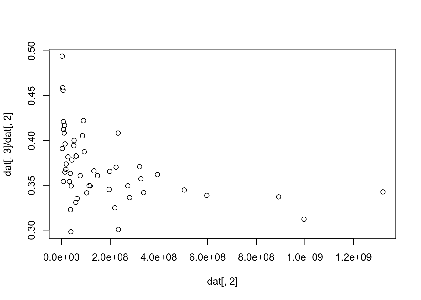
Miscellaneous graphing
After just a couple mistakes (not shown, e.g., col.text) this works to customize axes. The goal would almost never be to do this, but instead this was meant to show which argument highlighted which feature. Feel free to slap either of these on a graph. `axis(1, col = “red”, col.ticks = “yellow”), oraxis(1, col = “red”, col.ticks = “yellow”, col.axis = “blue”)``.
Corruption Index
None of this code works. Some of it generates output, some of it warnings, some of it errors. This is one of my least favorite things. We all have those. The goal was to reshape “wide” data into “long” data where we had columns for "Country", "Year", and "CPI". It’s somewhat offputting that the X is prepended to the year as a column name. Variable names can end, but not start, with numbers.
# dat2 <- read.delim("./data/cpi.csv")
# head(dat2)
# # oops sep = ','
# dat2 <- read.delim("./data/cpi.csv", sep = ',')
# head(dat2)
#
# reshape(dat2, varying = 2:ncol(dat2))
# reshape(dat2, varying = 2:ncol(dat2), direction = "long")
# ...
# redacted
# ...
Olympic athlete data
This excellent data comes from GitHub12. Below we will make a table of values of each sport entry. First is a plot() of a table(), then a barplot(), then finally the same barplot with rotated axes. These are all fine but could easily be made better.
athletes <- read.delim("./data/athletes.csv", sep = ",")
head(athletes)
id name nationality sex date_of_birth height weight
1 736041664 A Jesus Garcia ESP male 1969-10-17 1.72 64
2 532037425 A Lam Shin KOR female 1986-09-23 1.68 56
3 435962603 Aaron Brown CAN male 1992-05-27 1.98 79
4 521041435 Aaron Cook MDA male 1991-01-02 1.83 80
5 33922579 Aaron Gate NZL male 1990-11-26 1.81 71
6 173071782 Aaron Royle AUS male 1990-01-26 1.80 67
sport gold silver bronze info
1 athletics 0 0 0
2 fencing 0 0 0
3 athletics 0 0 1
4 taekwondo 0 0 0
5 cycling 0 0 0
6 triathlon 0 0 0 tab <- table(athletes$sport)
par(mfrow = c(3, 1))
barplot(tab)
plot(tab)
plot(tab, las = 3)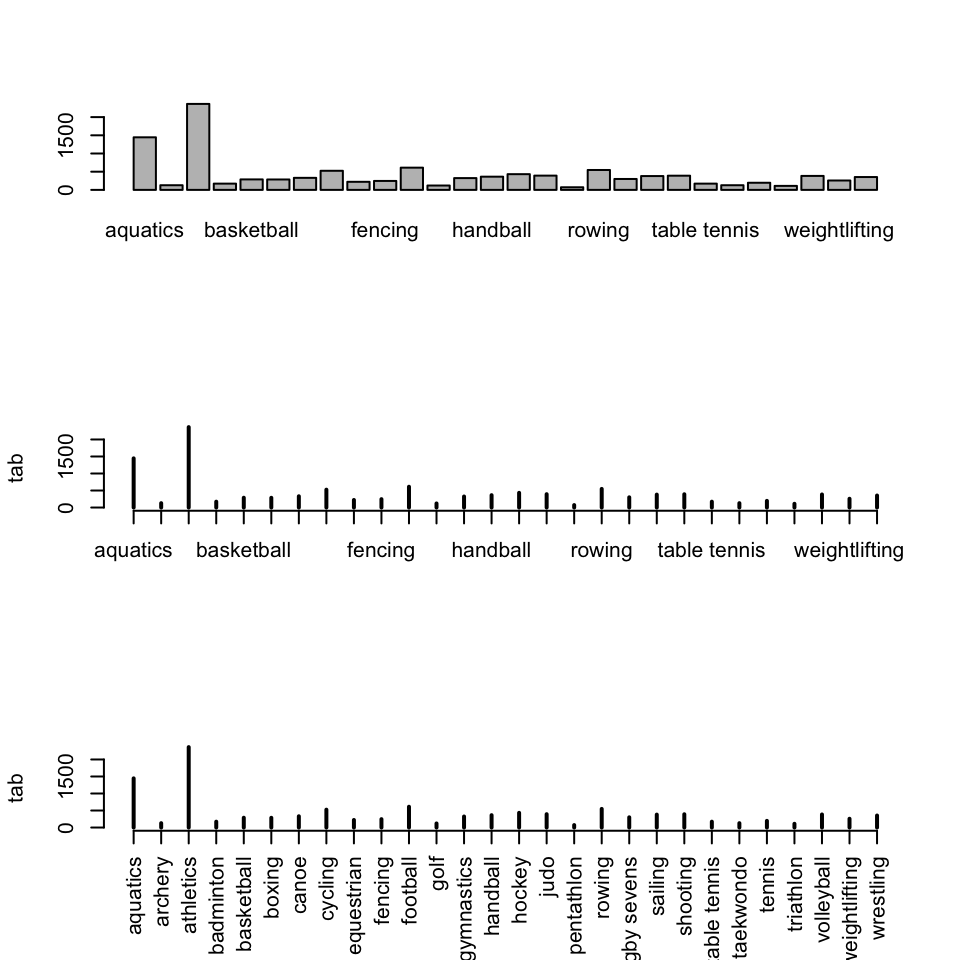
The table entries can be ordered (in either order), and the table replotted in a potentially nicer order. This would almost certainly break apart any sort of regional or alphabetical ordering (unless, “Which state is closest to the front of the alphabet?”). This rather quickly makes an excellent summary. It could be touched up a bit, two orientations and constructions are shown in Figure 2.
tab <- tab[order(tab)]
par(mfrow = c(1, 2))
barplot(tab, las = 1, horiz = TRUE)

plot(tab, las = 3)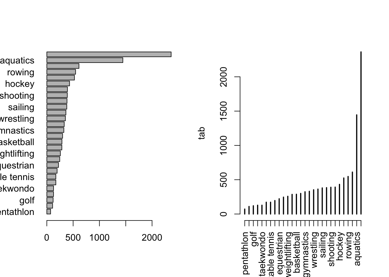
We’ve earlier looked at tasks like subsetting data, to create a data frame, you could estract the rows matching a condition by the following. This leads into a very interesting related task. Read ahead.
To save all columns of data for which the entries of athletes$nationality match "KOR" leave the second position empty. It would be nice to save this in a scheme similar to what you’re already doing, for me dat leads to dat.kor (if you felt like being annoying you could capitalize to dat.KOR, but if you capitalize that, why stop ? Just scream all of the time.).
dat.kor <- athletes[athletes$nationality == "KOR", ]If you wanted to make a plot you could pull that subset in the plot.
plot(output ~ input, athletes, subset = nationality == "KOR")Either of those could be done with multiple logic conditions. By specifiying a column or more using any of those methods, you could extract any subset of columns at the step creating dat.kor.
On the topic of selecting certain subsets, there are some clever approaches below. We did this a while back, but remember tab?
tab <- tab[order(tab)]; tab
modern pentathlon         triathlon              golf           archery
               72               110               120               128
        taekwondo         badminton      table tennis            tennis
              128               172               172               196
       equestrian           fencing     weightlifting            boxing
              222               246               258               286
       basketball      rugby sevens        gymnastics             canoe
              288               300               324               331
        wrestling          handball           sailing        volleyball
              353               363               380               384
         shooting              judo            hockey           cycling
              390               392               432               525
           rowing          football          aquatics         athletics
              547               611              1445              2363
Suppose we wanted the top ten sports by “abundance”. Looking at our table, in particular its dimensions, this is the entries 19:28 (in front of people you should always check your math 19:28 is of length 10).
tab[19:28]
   sailing volleyball   shooting       judo     hockey    cycling     rowing
       380        384        390        392        432        525        547
  football   aquatics  athletics
611 1445 2363 names(tab[19:28]) [1] "sailing" "volleyball" "shooting" "judo" "hockey"
[6] "cycling" "rowing" "football" "aquatics" "athletics" In the second line we pull off the names (you can verify its output). Next we will search for which rows in the sport column have an entry matching a sport in at list. We can also do this in reverse, identifying sports not in the, by bracketing the logical test with a !().
Here we aren’t going to store data frames, but will show the dimensions of those matching various characteristics with respect to row and column selections. The “list search” operator searches its input against a each elemnt of a provided list.
dim(athletes[athletes$sport %in% names(tab[19:28]), ])[1] 7469 12dim(athletes[!(athletes$sport %in% names(tab[19:28])), ])[1] 4069 12For proof-of-concept, we can take subsets of columns as numbers or variable names.
dim(athletes[!(athletes$sport %in% names(tab[19:28])), 1:5])[1] 4069 5head(athletes[!(athletes$sport %in% names(tab[19:28])), 1:5]) id name nationality sex date_of_birth
2 532037425 A Lam Shin KOR female 1986-09-23
4 521041435 Aaron Cook MDA male 1991-01-02
6 173071782 Aaron Royle AUS male 1990-01-26
16 521036704 Abbie Brown GBR female 1996-04-10
17 149397772 Abbos Rakhmonov UZB male 1998-07-07
29 349871091 Abdelhafid Benchabla ALG male 1986-09-26head(athletes[!(athletes$sport %in% names(tab[19:28])), ]) id name nationality sex date_of_birth height
2 532037425 A Lam Shin KOR female 1986-09-23 1.68
4 521041435 Aaron Cook MDA male 1991-01-02 1.83
6 173071782 Aaron Royle AUS male 1990-01-26 1.80
16 521036704 Abbie Brown GBR female 1996-04-10 1.76
17 149397772 Abbos Rakhmonov UZB male 1998-07-07 1.61
29 349871091 Abdelhafid Benchabla ALG male 1986-09-26 1.86
weight sport gold silver bronze info
2 56 fencing 0 0 0
4 80 taekwondo 0 0 0
6 67 triathlon 0 0 0
16 71 rugby sevens 0 0 0
17 57 wrestling 0 0 0
29 NA boxing 0 0 0 There was interest in calculating age using the participant’s given birth year (and the date of the Olympics). You could convert both to julian dates and subtract.
Hepatitis
We read in the hepatitis data13 and demontrate the construction of a multidimensional table. Applying as.data.frame() to these results is usually very useful in small datasets, often to check for the presence of missing or unusual combinations of variables.
dat <- read.delim("./data/hepatitis.csv", sep = ",")
head(dat)
age sex steroid antivirals fatigue malaise anorexia liver_big liver_firm
1 30 male false false false false false false false
2 50 female false false true false false false false
3 78 female true false true false false true false
4 31 female true false false false true false
5 34 female true false false false false true false
6 34 female true false false false false true false
spleen_palpable spiders ascites varices bilirubin alk_phosphate sgot albumin
1 false false false false 1.0 85 18 4.0
2 false false false false 0.9 135 42 3.5
3 false false false false 0.7 96 32 4.0
4 false false false false 0.7 46 52 4.0
5 false false false false 1.0 NA 200 4.0
6 false false false false 0.9 95 28 4.0
protime histology class
1 NA false live
2 NA false live
3 NA false live
4 80 false live
5 NA false live
6 75 false livetable(dat[, c("steroid", "antivirals", "fatigue")]), , fatigue =
antivirals
steroid false true
0 0
false 1 0
true 0 0
, , fatigue = false
antivirals
steroid false true
0 1
false 13 7
true 31 2
, , fatigue = true
antivirals
steroid false true
0 0
false 49 6
true 37 8That’s all for now.
Footnotes
I have a suspicion that
tab-is a useful code chunk label for referencing, but I never really care about showing this so the labeling is secondary for me. I’m almost 100% sure I’m wrong. Some things never change.↩︎You may also bounce to the fancier tools in a couple of weeks, but, oh well, at least you’ll have some perspective. “Oh, that was terrible,” is ok sometimes.↩︎
Things could go off the rails here in terms of a philosophical thing that I am too tired for.↩︎
As a weird aside, it is quite tricky to do this one by column numbers without some clumsy side-stepping.↩︎
This is a time to be creative. There was a time where I was very excited about Big Data, but it’s always the case that despite best interests, people always seem to have small data and quirks of them all are worth the individual attention.↩︎
Homework.↩︎
... all.x = <T/F>...,'...all.y=<T/F>...or some combination↩︎It had its faults, but generally it did a lot of good.↩︎
Eek.↩︎
The dig was at myself. I’d made a bet that I could get by without saying the name
iris.↩︎I’ll have to check the source.↩︎