wk2-followup-work

Introduction

Milestones of adulthood

Read in the data in milestone.csv stored in the folder data/.

Use the code chunk below as a start. Code chunks can be lengthy or brief.

dat <- read.delim(file="./data/milestone.csv", header = TRUE, sep = ',')
head(dat, n = 5)

    milestone year percent
1 independent 1983      83
2 independent 1993      77
3 independent 2003      77
4 independent 2013      73
5 independent 2023      64

tail(dat, n = 8)

   milestone year percent
13     child 2003      55
14     child 2013      50
15     child 2023      35
16      home 1983      49
17      home 1993      42
18      home 2003      44
19      home 2013      35
20      home 2023      33

This is the graph we ended class with.

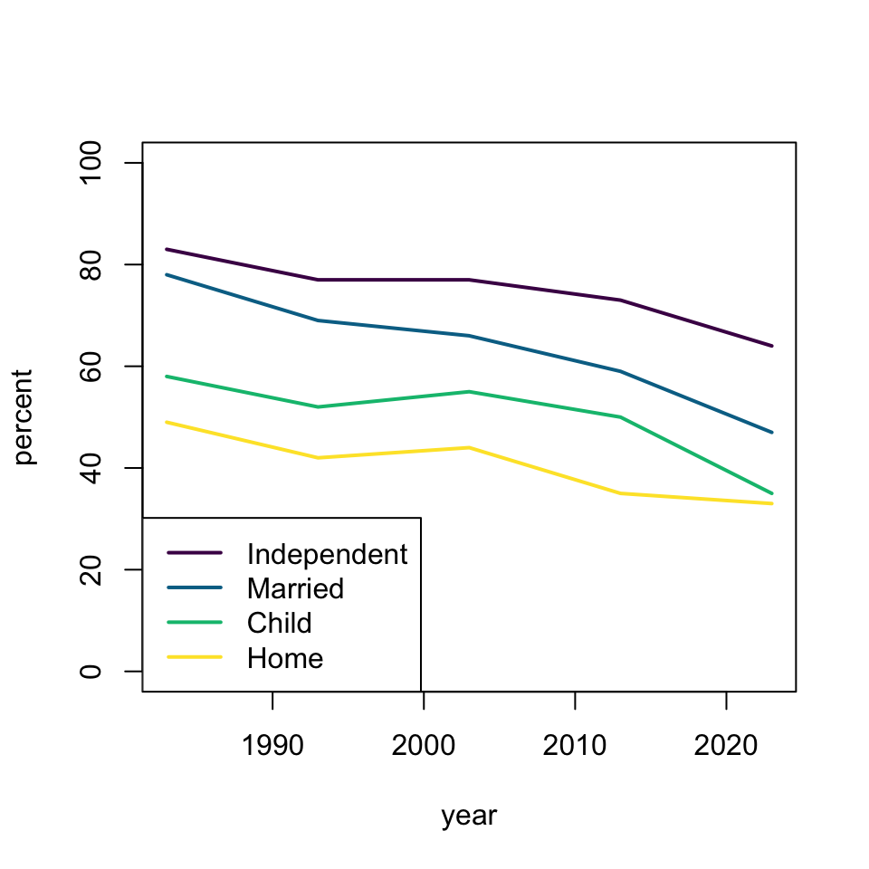
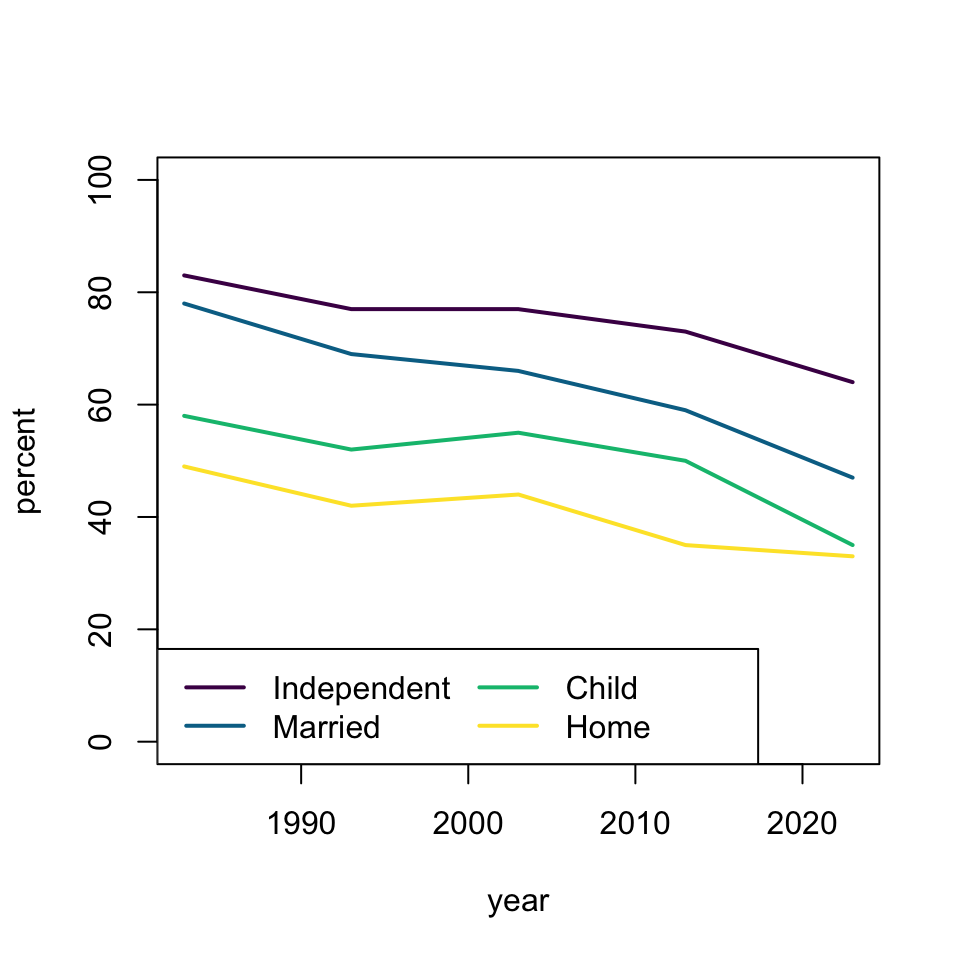
plot(percent ~ year, dat, subset = milestone == "independent", ylim = c(0, 100), type = 'l', lwd = 2, col = hcl.colors(4)[1])
lines(percent ~ year, dat, subset = milestone == "married", type = 'l', lwd = 2, col = hcl.colors(4)[2])
lines(percent ~ year, dat, subset = milestone == "child", type = 'l', lwd = 2, col = hcl.colors(4)[3])
lines(percent ~ year, dat, subset = milestone == "home", type = 'l', lwd = 2, col = hcl.colors(4)[4])
legend("bottomleft", c("Independent", "Married", "Child", "Home"), lty = 1, lwd = 2, col = hcl.colors(4))

Figure 1: Connected line graphs for percent of target population meeting four independently-determined metrics of adulthood, by UC Census Bureau data.

Other implementations or visualizations

Using base R commands the approach below is a clever way to layer plots. The initial plot command plots one level of the data and sets all of the plot window options. The for loop, over the remaining choices of milestone values, addes lines for each corresponding level. Perhaps as it should be, the legend is written manually.

It is possible to create a vector of labels or phrases that could be used as main titles in the 2-by-2 layout (or recycled to provide the legend labels). Where miles was computed using the unique entries of the milestone variable, we could simply list the test as we wanted it to appear (as we did in the legend). To use those entries, for ecample as main = labs[i] we would just index by the position of the label we wanted.

It is possible to use text-based labels for the lines directly, but in doing that we would want to be very careful of using yellow text on white. This could be done with clever applications of text() and some editing of the plot margin or axes limits.

Modify the code below to include more pleasing axes labels and tick mark labels that better align with the underlying data.

(miles <- unique(dat$milestone))

[1] "independent" "married"     "child"       "home"       

plot(percent ~ year, dat, subset = milestone == miles[1], ylim = c(0, 100), type = 'l', lwd = 2, col = hcl.colors(4)[1])

for(i in 2:length(miles)){
  lines(percent ~ year, dat, subset = milestone == miles[i], type = 'l', lwd = 2, col = hcl.colors(4)[i])
}
legend("bottomleft", c("Independent", "Married", "Child", "Home"), lty = 1, lwd = 2, col = hcl.colors(4), ncol = 2)

Figure 2: Connected line graphs for percent of target population meeting four independently-determined metrics of adulthood, by UC Census Bureau data.

A scatterplot

Make the graph above, but this time as a scatterplot with a relevant legend. The legend should show the point(s), not line segments. This is similar to how you could make scatterplots of raw data, modifying point or color by the value of some categorical variable. Again, we will see alternative approaches soon using ggplot().

Modify the code above to produce a scatterplot. Be sure to give this code chunk a distinct name.